The basics
Model structure
Hydrobricks models are built from three kinds of objects: bricks, processes, and fluxes.
A brick is any storage that holds water — a snowpack, a glacier, a soil reservoir, and so on. Each brick can contain multiple water containers: the snowpack, for instance, tracks snow and liquid water separately.
A process extracts water from a brick. Snowmelt, evapotranspiration (ET), and reservoir outflow are all processes. Each brick can have one or more processes assigned to it.
A flux carries extracted water somewhere: to another brick, to the atmosphere, or to the basin outlet. Together, bricks, processes, and fluxes form a directed water-transport graph that is solved at each time step.
Currently, only pre-built model structures are available. An instance is created by calling the model class with the desired options:
socont = models.Socont(soil_storage_nb=2)
The available models and their options are described on the models page.
Inspecting the structure
The structure of a model can be inspected right after construction (no setup() or
run() needed). It reflects the complete structure, including the auto-generated parts
(snow routine, precipitation splitters, forest canopy, glacier reservoirs), and each flux
is labelled with the process that withdraws the water.
model = models.HBV96()

# Textual summary (à la model.summary() in deep-learning frameworks)
model.print_structure()

# A serializable graph object
graph = model.get_structure_graph()
graph.to_dict()      # nested dict (nodes + edges)
graph.to_json()      # JSON string
graph.to_yaml()      # YAML string
graph.to_dot()       # Graphviz DOT string (no extra dependency)

# A rendered diagram (requires the optional `graphviz` package)
model.plot_structure('model_structure', fmt='png')
The diagram can be tuned with several options (also available on
graph.plot() / graph.to_dot()):
model.plot_structure(
    'model_structure',
    fmt='pdf',           # 'png', 'pdf' or 'svg' ('pdf'/'svg' are vector = sharpest)
    dpi=200,             # raster resolution for PNG (default 150); ignored for vector
    with_forcing=False,  # drop the meteo forcing inputs for a cleaner diagram
    legend=False,        # omit the legend
    nodesep=0.8,         # spacing between nodes in a rank
    ranksep=1.0,         # spacing between ranks
    structure_id=2,      # which structure variant to draw
)
Models with glacier or lake covers define several structure variants (e.g. a
glacier-free base and a with-glacier variant); pass structure_id= to inspect a
specific one. with_forcing is also available on get_structure_graph().
Spatial structure
The Catchment object
Catchment is the central object for defining the study area. It is
initialized with a catchment outline shapefile and then provides access to the
DEM, hydro unit properties, and the preprocessing sub-modules:
catchment.topography— slope, aspect, hillshade (see Catchment topography)catchment.discretization— splitting the catchment into hydro units (see Catchment discretization)catchment.connectivity— lateral connectivity between units (see Catchment connectivity)catchment.solar_radiation— potential direct solar radiation (see Potential solar radiation)
import hydrobricks as hb

catchment = hb.Catchment(outline='path/to/watershed.shp')
catchment.extract_dem('path/to/dem.tif')
Catchment can also be used as a context manager to ensure file handles are
released automatically when preprocessing is complete:
with hb.Catchment(outline='path/to/watershed.shp') as catchment:
    catchment.extract_dem('path/to/dem.tif')
    ...
See the API reference for the full method list.
Hydro units
The catchment is discretized into sub-units called hydro units, which can represent elevation bands, hydrological response units (HRUs), raster pixels, or any other spatial partition. Hydro units can be defined in two ways: loaded from a CSV file, or generated automatically from a DEM.
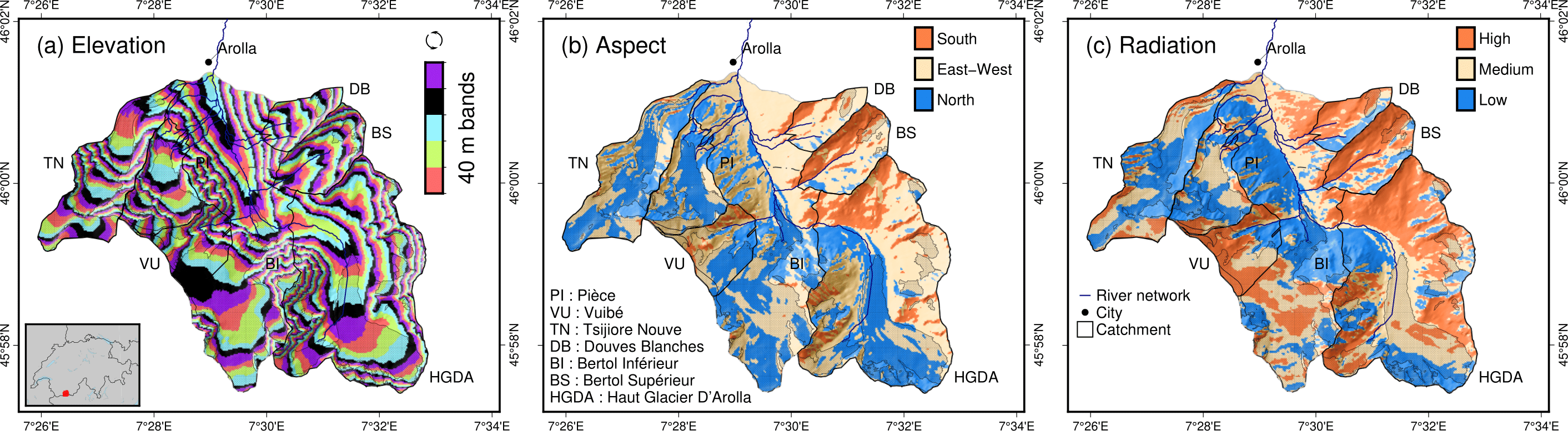
Example of discretization of a catchment based on (a) elevation bands, (b) aspect, and (c) potential solar radiation. Aspect or potential solar radiation is then combined with elevation bands to form hydro units. Source: Argentin et al. [2025]
Loading hydro units from a CSV file
The simplest way to define hydro units is to load them from a CSV file. At minimum, the file must contain the area and mean elevation of each unit:
hydro_units = hb.HydroUnits()
hydro_units.load_from_csv(
   'path/to/file.csv',
   column_elevation='elevation',
   column_area='area'
)
The CSV must have two header rows: the first with column names, the second with units. A minimal example:
num, elevation, area
-, m, m^2
0, 790, 2457500
1, 840, 4481250
2, 890, 5630625
3, 940, 5598125
4, 990, 4551250
5, 1040, 4579375
6, 1090, 4128125
7, 1140, 4807500
8, 1190, 4643750
9, 1240, 4662500
10, 1290, 4158750
11, 1340, 3496875
12, 1390, 2361250
By default, each hydro unit has a single open land cover. Catchments
with glaciers or other distinct surface types require multiple land covers.
Each land cover has a type (which determines its physical behaviour) and a
name (which distinguishes it from other land covers of the same type).
The available land cover types are:
open(aliasesground,generic,generic_land_cover): the default soil-bearing surface — the HBV “open areas” class; its behaviour comes entirely from the processes the model attaches to it. (groundwas the former default and is kept as an alias for backward compatibility.)glacier: a glacierized surface with ice melt, handled by the model’s glacier module (e.g. draining to dedicated reservoirs).forest: a soil-bearing surface that can optionally intercept rain in a canopy store (HBV only, enabled withforest_interception=True; see HBV land covers).lake: an exclusive open-water surface — all precipitation enters the open water, which evaporates at the potential rate and drains through a linear outflow (HBV only).
Which types a given model accepts depends on the model (see Models);
all models support open and glacier. For example, a catchment with bare-ice
and debris-covered glacier areas uses three land covers:
land_cover_names = ['open', 'glacier_ice', 'glacier_debris']
land_cover_types = ['open', 'glacier', 'glacier']

hydro_units = hb.HydroUnits(land_cover_types, land_cover_names)
hydro_units.load_from_csv(
   'path/to/file.csv',
   column_elevation='Elevation',
   columns_areas={
      'open': 'Area Non Glacier',
      'glacier_ice': 'Area Ice',
      'glacier_debris': 'Area Debris'
   }
)
The CSV must list the area of each land cover per hydro unit (more information in the Python API):
Elevation, Area Non Glacier, Area Ice, Area Debris
m, km2, km2, km2
3986, 2.408, 0, 0
4022, 2.516, 0, 0
4058, 2.341, 0, 0.003
4094, 2.351, 0, 0.006
4130, 2.597, 0, 0.01
4166, 2.726, 0, 0.006
4202, 2.687, 0, 0.061
4238, 2.947, 0, 0.065
4274, 2.924, 0.013, 0.06
4310, 2.785, 0.019, 0.058
4346, 2.578, 0.052, 0.176
4382, 2.598, 0.072, 0.369
4418, 2.427, 0.129, 0.384
4454, 2.433, 0.252, 0.333
4490, 2.210, 0.288, 0.266
4526, 2.136, 0.341, 0.363
4562, 1.654, 0.613, 0.275
Generating hydro units from a DEM
When spatial data are available, hydro units can be generated automatically from a DEM, with discretization criteria chosen to match the melt model in use:
Elevation only — sufficient for
'degree_day'Elevation + aspect — required for
'degree_day_aspect'Elevation + radiation — recommended for
'temperature_index'
See melt models for a description of each.
The following example discretizes a study area into 50 m elevation bands combined with aspect classes. The elevation range covers the entire catchment (1912–2893 m), with some margin added for the bands:
study_area = catchment.Catchment(outline='path/to/watershed/shapefile.shp')
success = study_area.extract_dem('path/to/dem.tif')
study_area.discretize_by(
   ['elevation', 'aspect'],
   elevation_method='equal_intervals',
   elevation_distance=50,
   min_elevation=1900,
   max_elevation=2900,
)
Discretizing by potential solar radiation
The 'temperature_index' melt model requires per-unit radiation values.
Hydrobricks computes the daily mean potential clear-sky direct solar radiation
at the DEM surface [W/m²] using the equation of Hock [1999]. The radiation
resolution defaults to the DEM resolution; for high-resolution DEMs, specify
a coarser resolution to keep computation times reasonable.
study_area = catchment.Catchment(outline='path/to/watershed/shapefile.shp')
success = study_area.extract_dem('path/to/dem.tif')
study_area.calculate_daily_potential_radiation('path/to/file', resolution)
Because radiation depends only on topography, not on the simulation year, the
result can be saved to a GeoTIFF and reloaded in future runs. The default
filename is 'annual_potential_radiation.tif':
study_area = catchment.Catchment(outline='path/to/watershed/shapefile.shp')
success = study_area.extract_dem('path/to/dem.tif')
study_area.load_mean_annual_radiation_raster(
   'path/to/file',
   filename='annual_potential_radiation.tif'
)
With the radiation loaded, pass it as a discretization criterion:
study_area.discretize_by(
   ['elevation', 'radiation'],
   elevation_method='equal_intervals',
   elevation_distance=50,
   min_elevation=1900,
   max_elevation=2900,
   radiation_method='equal_intervals',
   radiation_distance=65,
   min_radiation=0,
   max_radiation=260
)
Running the model
Once you have defined the hydro units, parameters, and forcing, set up and run the model:
socont.setup(
   spatial_structure=hydro_units,
   output_path='/path/to/dir',
   start_date='1981-01-01',
   end_date='2020-12-31'
)

socont.run(parameters=parameters, forcing=forcing)
The outlet discharge (in mm/d) can then be retrieved:
sim_ts = socont.get_outlet_discharge()
To export all internal fluxes and states to a NetCDF file for further analysis:
socont.dump_outputs('/output/dir/')
Initializing state variables
By default, all water storages (snowpack, soil reservoirs, etc.) start empty at
the beginning of the simulation. To initialize them to more realistic values,
call initialize_state_variables() between setup() and run():
socont.initialize_state_variables(
   parameters=parameters,
   forcing=forcing
)
socont.run(parameters=parameters, forcing=forcing)
This runs the model once over the full simulation period, captures the final storage values, and uses them as the starting point for subsequent runs. When the model is run multiple times — as during calibration — it resets to these saved values at the start of each run rather than to empty reservoirs.
Spin-up and warmup
The very first years of a simulation are typically unreliable because the storages start empty and have not yet settled into a realistic seasonal cycle. Two mechanisms address this:
Spin-up (recommended). Pass spinup to setup() and the model replays
the first years of its own period (without logging) to initialize the storages,
then restarts at the period start with the warmed-up states:
socont.setup(
   spatial_structure=hydro_units,
   output_path='/path/to/dir',
   start_date='1981-01-01',
   end_date='2020-12-31',
   spinup='4y',   # or a number of days, e.g. 1461
)
The spin-up happens transparently on every run (including each calibration
run), no forcing data before start_date is needed, and the whole
declared period can be evaluated — no year of observations is discarded. The
land cover area fractions are restored to their initial values after the
spin-up (only the storage states are kept), and a spin-up longer than the
period is clamped to a single replay of the whole period.
Warmup trimming (legacy alternative). Without a spin-up, the opening period
of each run can instead be excluded from the evaluation: the calibration setup
accepts a warmup argument (in days) for this purpose — see the
calibration page. The evaluated span is then shorter than
the declared one.
Evaluation
After a run, performance metrics can be computed by comparing the simulated discharge to observations. Load observations from a CSV file (discharge in mm/d):
obs = hb.Observations()
obs.load_from_csv(
   '/path/to/obs.csv',
   column_time='Date',
   time_format='%d/%m/%Y',
   content={'discharge': 'Discharge (mm/d)'}
)
obs_ts = obs.data[0]

nse = socont.eval('nse', obs_ts)
kge_2012 = socont.eval('kge_2012', obs_ts)
Metrics are provided by the HydroErr package. Any metric from their full list can be used by passing its function name as a string.
eval() also accepts a period to score a date slice of the simulation
only (e.g. a validation period), and a whole simulation can be scored on
several declared periods at once with evaluate_periods() — see
calibration and validation periods.
Outputs
Results are available at three levels of detail:
Direct outputs — scalar or time-series summaries available immediately after a run.
A NetCDF output file — per-hydro-unit fluxes and states, exported on demand.
Auxiliary files — spatialized forcing, log files, and calibration records.
Direct outputs
The following outputs are accessible on the model object after a run:
Time series:
get_outlet_discharge(): daily discharge at the basin outlet (mm/d)
Integrated totals over the simulation period:
get_total_outlet_discharge(): total discharge at the outletget_total_et(): total evapotranspirationget_total_water_storage_changes(): net change in total water storage from the start to the end of the simulationget_total_snow_storage_changes(): net change in snow storage
NetCDF output file
A detailed NetCDF file is exported with model.dump_outputs('some/path').
How much data it contains depends on the record_all option set at model
creation:
record_all=False(default): only outlet discharge and a few selected time series are stored. Use this during calibration.record_all=True: every flux and state variable is recorded at every time step. This is useful for diagnosing model behaviour but slows execution and produces large files.
Recording specific stores and fluxes
When only a few internal series are needed — for example an auxiliary calibration
signal such as glacier mass balance — recording everything with record_all=True
is wasteful. Instead, record just the required items. The recordings must be configured
before model.setup() (they are part of the model build).
An auxiliary observation knows what it needs; let it configure the model for you:
glacier_mb.configure_recording(model)   # before model.setup()
model.setup(...)
To record specific items by hand, build a
RecordingRequest and pass it to
model.add_recordings:
from hydrobricks.evaluation import RecordingRequest

model.add_recordings(RecordingRequest(
    brick_states=[('glacier_snowpack', 'snow_content')],   # '<brick>:<item>'
    process_outputs=[('glacier', 'melt', 'output')],       # '<brick>:<process>:<item>'
    fractions=True,                                        # land-cover fractions over time
))
model.setup(...)
The recorded series are read from memory (model.get_recorded_hydro_unit_values(label))
or written to the NetCDF output, exactly like those from record_all.
File structure
Dimensions:
time: the temporal axishydro_units: one entry per hydro unit (e.g., per elevation band)aggregated_values: catchment-scale (lumped) quantitiesdistributed_values: per-hydro-unit quantitiesland_covers: one entry per land cover
Global attributes that map variable indices to names:
labels_aggregated: names of lumped elements (fluxes and states)labels_distributed: names of distributed elementslabels_land_covers: names of land covers
To inspect the available labels:
results = hb.Results('path/to/netcdf_results_file')
print(results.results.attrs)
Example output for GSM-Socont with two glacier types:
labels_aggregated =
   "glacier_area_rain_snowmelt_storage:content",
   "glacier_area_rain_snowmelt_storage:outflow:output",
   "glacier_area_icemelt_storage:content",
   "glacier_area_icemelt_storage:outflow:output",
   "outlet";

labels_distributed =
   "open:content",
   "open:infiltration:output",
   "open:runoff:output",
   "glacier_ice:content",
   "glacier_ice:outflow_rain_snowmelt:output",
   "glacier_ice:melt:output",
   "glacier_debris:content",
   "glacier_debris:outflow_rain_snowmelt:output",
   "glacier_debris:melt:output",
   "open_snowpack:content",
   "open_snowpack:snow",
   "open_snowpack:melt:output",
   "glacier_ice_snowpack:content",
   "glacier_ice_snowpack:snow",
   "glacier_ice_snowpack:melt:output",
   "glacier_debris_snowpack:content",
   "glacier_debris_snowpack:snow",
   "glacier_debris_snowpack:melt:output",
   "slow_reservoir:content",
   "slow_reservoir:et:output",
   "slow_reservoir:outflow:output",
   "slow_reservoir:percolation:output",
   "slow_reservoir:overflow:output",
   "slow_reservoir_2:content",
   "slow_reservoir_2:outflow:output",
   "surface_runoff:content",
   "surface_runoff:outflow:output";

labels_land_covers =
   "open",
   "glacier_ice",
   "glacier_debris";
Variables in the file:
time(1D): dates as Modified Julian Dates (days since 1858-11-17 00:00)hydro_units_ids(1D): IDs of the hydro unitshydro_units_areas(1D): area of each hydro unit [m²]sub_basin_values(2D): lumped time series, indexed bylabels_aggregatedhydro_units_values(2D): distributed time series, indexed bylabels_distributed. Two important subtypes:Flux variables (names ending in
:output, unit: mm): already weighted by land cover fraction and relative hydro unit area. You can sum them directly over all hydro units to get the catchment-total contribution of a component (e.g., total glacier melt).State variables (names ending in
:contentor:snow, unit: mm): the water depth stored in a reservoir. These are not area-weighted — to aggregate over the catchment, multiply each value by its land cover fraction and relative hydro unit area. TheResultsclass provides helpers that do this for you:get_mean_hydro_units_values()(area-weighted catchment mean of any component for one land cover),get_land_cover_areas()(per-unit area of a land cover over time), and, specifically for snow water equivalent,get_total_swe()(per-unit SWE aggregated across all land covers) andget_mean_swe()(the catchment-wide mean). Land covers without a snowpack (e.g. open water) contribute zero SWE over their area.
land_cover_fractions(2D, optional): time series of land cover fractions, present when glacier or other land cover evolution is active.
Auxiliary outputs
Spatialized forcing (
forcing.nc): the per-unit forcing time series, saved withforcing.create_file(). Useful for inspecting what the model actually received as input.Log files (
hydrobricks_...log): execution logs that record warnings and errors, useful for debugging.Hydro units raster (
hydro_units.tif): a GeoTIFF with unit IDs as pixel values, useful for spatial visualization.Hydro units table (
hydro_units.csv): unit properties (elevation, area, land cover fractions) in tabular form.Annual radiation raster (
annual_potential_radiation.tif): potential clear-sky solar radiation, saved during preprocessing.Calibration records: SPOTPY saves every model evaluation to CSV or SQL during calibration.